记录在用Python重写吴恩达（Andrew Ng）的机器学习（Machine Learning | Coursera）的课后练习的过程中遇到的一些问题（另，吴恩达在 Coursera 上的机器学习的 python 版本的代码挂在了github上：ML-EX-Python）

一、Numpy篇

1.(m,)和(m,1)的区别

假设load一个数据集时，得到一个97x2的矩阵，设为data1. 对data1作 data1[:, 0] 切片，得到的矩阵的shape将是(97,)，在我的理解里~~这是一个1x97的矩阵（也可以说是行向量），在需要时要reshape成(97,1)的97x1的列向量~~。

2018年11月6日补充：shape为 (m,) 这类的矩阵，根据恩达 “ 2.16 关于 python / numpy 向量的说明 ” 一节视频中说道，这类矩阵称为 " rank 1 array " （秩为1的数组），既不是行向量也是列向量。

2.axis与多维矩阵

对于2维矩阵，axis = 0 和 axis = 1 分别代表着沿列和沿行进行的动作。例如：

a = np.array([[1, 2], [3, 4]])
b = np.array([[5, 6], [7, 8]])
# a.shape : (2,2)  a.ndim : 2
c = np.append(a, b, axis=0)
d = np.append(a, b, axis=1)
print(c)
print(d)

###############################
[[1 2]
 [3 4]
 [5 6]
 [7 8]]

[[1 2 5 6]
 [3 4 7 8]]
###############################

而对于三维矩阵，我是这么理解的：假设有一个三维矩阵：

f = np.array([[[0, 1], [2, 3], [2, 7]], [[2, 1], [4, 4], [1, 3]], [[2, 1], [2, 0], [4, 6]]])
# f.shape : (3,3,2)  f.ndim : 3

将他看做是一个3x3的矩阵，3x3就是 f.shape 的前两个，这个3x3的二维矩阵的第一个3代表着f这个三维矩阵的层数，第二个3（既这个二维矩阵的列）代表着每一层的行数，相当于这个二维矩阵的每一个元素（共9个元素）都是一个长度为2的向量，例如第0层第0号元素是[0, 0]. 用求和来解释一下 axis = 1/2/3 的三种情况的区别：

print(np.sum(f, axis=0))

[[ 4  3]
 [ 8  7]
 [ 7 16]]

print(np.sum(f, axis=1))

[[ 4 11]
 [ 7  8]
 [ 8  7]]

print(np.sum(f, axis=2))

[[ 1  5  9]
 [ 3  8  4]
 [ 3  2 10]]

axis等于0的时候，既做的沿列方向的求和，既把列方向上的所有元素（每个元素又都是一个长度为2的向量）相加，例如这个二维数组的列方向求和中的第一列就是(0,1)、(2,1)、(2,1)，相加后既(4,3)，以此类推。

axis等于1的时候，同上。

axis等于2的时候，相当于求出这个二维的3x3的矩阵中每个元素的和，（既三维矩阵中每一层中每一行的值），用图表示就是：

3.np.std()算出来的标准差和Octave、Matlab不一样

np.std()算的标准差默认是样本标准差，也就是分母为n-1个自由度的。而想求分母的自由度为n的总体标准差，需要加上参数ddof，例如：

sigma = np.std(x, axis=0, ddof=1)

对于什么时候求样本标准差什么时候求总体标准差：如果求的是样本本身的真实标准差，那么既求总体标准差；若要用样本标准差去估计总体标准差时，既样本估计总体，例如有100个人的数据，想求整体（例如5万人）的标准差，那么就求样本标准差。

4.reshape中的order的使用

在numpy的reshape中，order的取值根据官网文档有：

order : {‘C’, ‘F’, ‘A’}, optional

默认是以'C'为序，既以行为序，例如：

a = np.arange(16)
print(a)
# [ 0  1  2  3  4  5  6  7  8  9 10 11 12 13 14 15]
print(np.arange(16).reshape(4, 4))
# [[ 0  1  2  3]
#  [ 4  5  6  7]
#  [ 8  9 10 11]
#  [12 13 14 15]]

但是若以'F'为序的话会是这样的（这也是matlab或octave中的reshape）：

b = np.arange(16).reshape(4, 4, order='F')
print(b)
# [[ 0  4  8 12]
#  [ 1  5  9 13]
#  [ 2  6 10 14]
#  [ 3  7 11 15]]

参照 How does numpy.reshape() with order = 'F' work? 的回答，可以这么理解：reshape函数会用指定的order先对矩阵进行ravel既化为1维，然后再根据同样的order进行排列。如下：

a = np.arange(16).reshape(4, 4)
# [[ 0  1  2  3]
#  [ 4  5  6  7]
#  [ 8  9 10 11]
#  [12 13 14 15]]
c = a.ravel(order='F')
print(c)
# [ 0  4  8 12  1  5  9 13  2  6 10 14  3  7 11 15]

再对新的这个1维数组做reshape，要注意的是，这时候的reshape的order也是'F'，例如若要重整为2x8的矩阵，那么这时候先取第1个值0，再跳2个值取8，再跳两个值1，反复到取到8个值，再反复做下一行。所以：

d = c.reshape(2, 8, order='F')
print(d)
# [[ 0  8  1  9  2 10  3 11]
#  [ 4 12  5 13  6 14  7 15]]

这等同于：

print(np.arange(16).reshape((4, 4)).reshape((2, 8), order='F'))
# [[ 0  8  1  9  2 10  3 11]
#  [ 4 12  5 13  6 14  7 15]]

5.用@contextmanager管理打印参数

在同段程序里打印不同参数的结果，例如某一次打印需要控制小数点位数，但在这之前的打印和之后的打印都不需要控制或者每次的参数都不同，那么可以由上下文进行方便的管理：

@contextmanager
def precision_print(precision=3):
    original_options = np.get_printoptions()
    np.set_printoptions(precision=precision, suppress=True)
    try:
        yield
    finally:
        np.set_printoptions(**original_options)

with precision_print(precision=3):
    print('Sigmoid gradient evaluated at [-1 -0.5 0 0.5 1]:\n %s \n\n' % g)

6.where的返回值多出一行向量

where其实相当于返回的是满足条件的数的坐标，所以如果对一个一维矩阵和对一个向量做where返回的值是不同的：

print(y.shape)
# (51, 1)
print(np.where(y == 1))
# (array([ 0,  1,  2,  3,  4,  5,  6,  7,  8,  9, 10, 11, 12, 13, 14, 15, 16,
       17, 18, 19, 50], dtype=int64), array([0, 0, 0, 0, 0, 0, 0, 0, 0, 0, 0, 0, 0, 0, 0, 0, 0, 0, 0, 0, 0],
      dtype=int64))
print(y[:, 0].shape)
# (51,)
print(np.where(y[:, 0] == 1))
# (array([ 0,  1,  2,  3,  4,  5,  6,  7,  8,  9, 10, 11, 12, 13, 14, 15, 16,
       17, 18, 19, 50], dtype=int64),)

7.数组类型为UINT8时要注意负号的使用

按道理，用下面两个式子肯定是一样的：

cost = np.sum((1 / m) * (-Y * np.log(A2) - (1 - Y) * np.log(1 - A2)))
cost = np.sum((-1 / m) * (Y * np.log(A2) + (1 - Y) * np.log(1 - A2)))

但是却发现两个式子求出来的结果不一样，是第一个式子求出来的结果错了。仔细排查计算流程后发现，这里的 Y 的类型是unit8，如果Y里有正数，以1为例，那么直接用 -Y 会得到255。所以这里应该用 (-1) * Y 或者把Y做类型转换。

8.pad的顺序理解

从axis上来说，先填0方向再填1方向，也就是先填列方向再填行方向。如果pad_width只填一组shape，则会自动用这组shape再填行方向。

二、Pandas篇

1.crosstab

前两个参数分别是index和columns，按index分组后统计columns里中的频数：

y_actu=np.array([6,2,3,4])
y_pred=np.array([1,2,1,5])
pd.crosstab(y_actu, y_pred, rownames=['Actual'], colnames=['Predicted'], margins=True)

Predicted  1  2  5  All
Actual                 
2          0  1  0    1
3          1  0  0    1
4          0  0  1    1
6          1  0  0    1
All        2  1  1    4

三、Matplotlib篇

1.plt.plot根据两点画图却看不到直线

plt.plot两点画线中的x和y要求的是向量，在这里可以理解成需要列向量而不能是横向量：

x.shape:(2,)    y.shape:(2,)   -->OK
x.shape:(2,1)   y.shape:(2,1)  -->OK
x.shape:(1,2)   y.shape:(1,2)  -->Not OK

2.散点图中画等高线时为等高线添加legend

在Stack Overflow上看了几个回答，加上“胡乱写了一下”发现下面这个对我有用，但是具体为什么可以起作用暂时没弄清楚：

plt.contour(u, v, z.T, [0]).collections[0].set_label("Decision boundary")

3.散点图中改marker的size和画空心圆marker

改marker的size以为参数名是 linewidths ，其实是 s ..

画空心圆其实就是改变圆心颜色和圆圈线条的颜色，分别由参数 c 和 edgecolors 控制，那么画空心圆就是把里面涂白、外面上色：( marker='o', c='', edgecolors='r' )

4.imshow中改变图片的size

尝试过xtick、figsize都不是想要的样子，然后找到了 figure of imshow() is too small - stackoverflow 这个问题，里面说道：

If you don't give an aspect argument to imshow, it will use the value for image.aspect in your matplotlibrc. The default for this value in a new matplotlibrc is equal. So imshow will plot your array with equal aspect ratio.

那就很清楚了，原来是长宽比固定了，那么只需要：

plt.imshow(Y, aspect='auto')

就能使图片以自动比例显示了，拉动figure的框也能自动放大缩小了。

四、其他

1.Matplotlib中cmap的取值

懒得每次去官网search：

cmaps = [('Perceptually Uniform Sequential', [
            'viridis', 'plasma', 'inferno', 'magma']),
         ('Sequential', [
            'Greys', 'Purples', 'Blues', 'Greens', 'Oranges', 'Reds',
            'YlOrBr', 'YlOrRd', 'OrRd', 'PuRd', 'RdPu', 'BuPu',
            'GnBu', 'PuBu', 'YlGnBu', 'PuBuGn', 'BuGn', 'YlGn']),
         ('Sequential (2)', [
            'binary', 'gist_yarg', 'gist_gray', 'gray', 'bone', 'pink',
            'spring', 'summer', 'autumn', 'winter', 'cool', 'Wistia',
            'hot', 'afmhot', 'gist_heat', 'copper']),
         ('Diverging', [
            'PiYG', 'PRGn', 'BrBG', 'PuOr', 'RdGy', 'RdBu',
            'RdYlBu', 'RdYlGn', 'Spectral', 'coolwarm', 'bwr', 'seismic']),
         ('Qualitative', [
            'Pastel1', 'Pastel2', 'Paired', 'Accent',
            'Dark2', 'Set1', 'Set2', 'Set3',
            'tab10', 'tab20', 'tab20b', 'tab20c']),
         ('Miscellaneous', [
            'flag', 'prism', 'ocean', 'gist_earth', 'terrain', 'gist_stern',
            'gnuplot', 'gnuplot2', 'CMRmap', 'cubehelix', 'brg', 'hsv',
            'gist_rainbow', 'rainbow', 'jet', 'nipy_spectral', 'gist_ncar'])]

除了这个还有各个图例的用法，也懒得每次都找：Gallery

2.一些小用法

def convert_to_one_hot(Y, C):
    Y = np.eye(C)[Y.reshape(-1)]
    return Y

Y_train = np.array([2,3,1])
Y_oh_train = convert_to_one_hot(Y_train, C=5)
#[[0. 0. 1. 0. 0.]
# [0. 0. 0. 1. 0.]
# [0. 1. 0. 0. 0.]]
#ndarray[[0]] is to select the first line in the ndarray

X_train = ['I am boy', 'I feel better now']
maxLen = len(max(X_train, key=len).split())
#maxLen = 4

vocab = dict()
vocab.update({'2': 0})
vocab.update({'4': 1})
string = "4142"
rep = list(map(lambda x: vocab.get(x, '<unk>'), string))
# [1, '<unk>', 1, 0]

3.Win10下安装tensorflow-gpu

安装日期为2019年3月19日。

刚好换了新的板U，顺便记录一下安装过程。参考官网安装教程和gpu支持。

1. 下载好 Anaconda3-5.2.0-Windows-x86_64.exe 然后安装，一路next，勾选 add to path 后install

~~（可省略?）2. 下载 cuda_10.1.105_418.96_win10.exe 并安装（cuda习惯性装在了C盘），自定义安装只选择CUDA~~

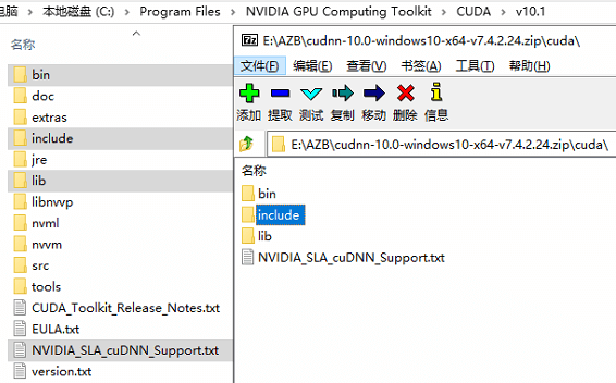
~~（可省略?）3. 下载 cudnn-10.0-windows10-x64-v7.4.2.24.zip 把里面的文件夹挪到cuda的安装目录下~~

4. 管理员打开anaconda prompt

conda create -n tfvenv python=3.6 tensorflow-gpu
conda activate tfvenv
//have a cup of coffee

安装TF的方式有很多，这里用的平时常用的（图省事）。看了下要安装的list，发现会再装一次cudatoolkit，应该可以省略第2、3步的（况且好像漏了把cuda kit加入path了），下次重装的时候再验证。

另外，如果没有指定python版本的话，会安装3.7，可能会导致 "Failed to load the native TensorFlow runtime."

OVER.

文章

Numpy、Pandas和Matplotlib的使用小结